GOTM
The General Ocean Turbulence model is both a state-of-the-art turbulence library for flows in natural waters and a 1D water column model.
GOTM was initiated by Hans Burchard and Karsten Bolding in 1998 and the first public release was in 1999. BB has always been responsible for maintaining the code – first using CVS and later using git. BB has provided numerous code contributions and has participated very active on the developers and users mailing lists.
The turbulence library of GOTM is used in a number of 3D ocean models - such as
GOTM is used as the primary test bed for Framework for Biogeochemical Models FABM.
GOTM has its own web-site where in-depth information can be found.
Here we will just provide some information on new features BB is doing on the core GOTM code. This does not include utilities described elsewhere on this site - but only changes to the core part of the GOTM source code. This is typically new features that requires a significant knowledge of the entire code base - but also quite some resources in terms of implementation and testing time.
Developments by BB
The table below describes the on-going GOTM developments at BB. As described here it is very difficult to get funding for pure model development. On the other hand - to bring things forward - you can’t wait for funding agencies to be ready.
BB has therefor initiated projects using BB resources - that hopefully someday can be released for general use - but it will require funds.
YAML Configuration
Rationale
Until now GOTM has been configured through a combination of namelists (in a number of files) and text files (scalar time-series and profiles). Namelists - being a standard Fortran feature - has clear advantages and replacing them with a costum configuration system must be carefully evaluated. The main disadvantage of namelists is - they are Fortran only - i.e. any manipulation of the namelists must be done either in an editor or through costum made tools (like editscenario). New use cases of GOTM - e.g. auto-calibration - requires a flexible easy maintainable system for generating ensembles of configurations in a non-interactive way. FABM and the output manager in GOTM already uses YAML as configuration format so replacing namelists with a YAML-formatted configuration file seems the obvious choice.
Implementation details
The implementation depends on the Fortran YAML library developed by Jorn Bruggeman and briefly described here.
To ease the transition from namelist based configuration to YAML-based a method for converting namelists to a YAML-file has been implemented via command line options as seen in the figure below.
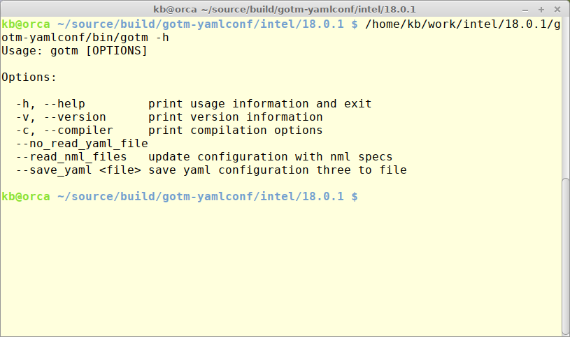
The default - calling GOTM executable without any options - will read gotm.yaml. Skipping reading gotm.yaml can be achieved by specifying –no_read_yaml_file. Reading an existing - working - namelist configuration can be done be specifying –read_nml_files. Saving the final configuration to a new YAML-formatted file can be done by specifying –save_yaml where file is the name of the target YAML file.
To create a starting point for a new configuration with default parameter settings the following command can be used: gotm –save_yaml default.yaml.
To convert an existing namelist based configuration use this command: gotm –read_nml_files –save_yaml gotm.yaml
Present status
The code is presently in a private BB development Gitlab repository. When feature complete the code will be moved to a public branch of the main GOTM Github repository for discussion and testing.
Presently output.yaml has not been merged with gotm.yaml - if it will depends on some further workflow experiences.
Output operators
The flexible output facility used in GETM and GOTM have changed the way output is done. Much of the work previously done as post-processing is now done as part of model simulation. This has advantages and dis-advantages. The main dis-advantage being that the wall clock time for a given simulation will increase - because of the extra work being done. This is, however, usually more than compensated by the reduced time in the normal post-processing. The main advantage is the flexibility introduced to the output specifications. A mix of resolutions in space and time for different output regions can be defined without having to save everything with the highest space and time resolution to accomplish all possible combinations - as has been the case until now. Have being used for some time in operational mode at FMI/GeoMETOC has made apparant the need for additional features in relation to 1) timing of calculations of derived fields and 2) a more flexible reference for the vertical coordinate used in the outputs.
Rationale
With the flexible output it is possible store any number of domains defined as hyper-slabs of the full domain in all 4 dimensions (x, y, z, t) through specifications in a YAML formatted file. This allows to e.g. save data from a station like region in high temporal resulution and on the other hand save the entire calculation domain in a reduced resultion to save space. Note that since any number of different outputs can be defined
Implementation details
The timing of calculations is implemented as an additional logical variable in the output Fortran class. During the integration the output manager sets the variable to true if the variable is to be stored in the present time step. The algorithm taking care of the calculation of the derived field will check the status of the variable - and if true do the calculation.
The output operators are implemented as a Fortran class library interacting with a field manager (to obtain meta-data for involved fields) and a YAML parsing library (for flexible configuration). Being a class library the functionality can easily be extended to include new operators without influencing the overall structure. Presently are implemented an interpolation operator that will do interpolation along a coordinate axis and a time averaging operator. The background for the operators is online conversion - and storage - of fields with geo-potential (z) coordinate from sigma-coordinate type of models.
Present status
The output operators have been merged into the master GOTM repository as of January 2019nd can be used by both GOTM and GETM. Below is an example of a GETM configuration defining a station type output interpolating the sigma-coordinate model field to a z-coordinate field using the sea surface a reference.
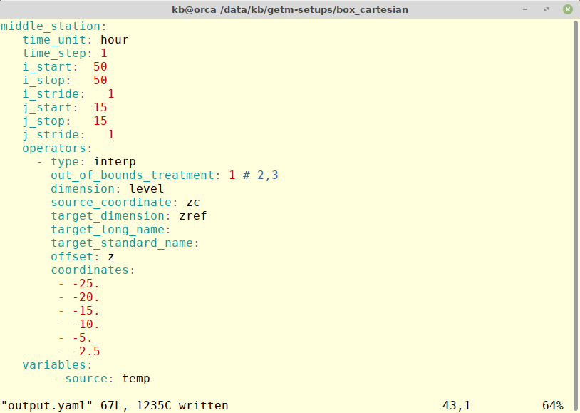
The example will create a file - middle_station.nc - where the temperature is saved every hour for the center positon in box_cartesian test case. The output will use the interp operator and store interpolated values at the coordinates given using the sea surface as reference (z). The out_of_bounds and target* variables are optional.
The short manual provided as part of the project can be download here.
Data Assimilation
Nothing yet
Hotstart
Rationale
Even though GOTM simulations typically executes quite fast there are use cases where dividing the simulation in parts do make sense. One example is when doing i a coupled physical/bio-geochemical simulation. It is desirable to have the i physical fields in balance before bio-geochemistry is switched on. A second example i is when doing ensemble data-assimilation studies. Here starting the simulation i from a analyzed state is mandatory.
Implementation details
The hotstart feature in GOTM is implemented on top if the field_manager utilising the possibility to add attributes to variables. For state variables – and other variables necessary to perform a hotstart – an extra attribute state is added during registration in the field_manager. The output_manager utilizes the state attribute information when creating a list of fields that must be either written to - or read from - the hotstart file. The link to the data in the NetCDF formatted hotstart file is done through the name variable in the field_manager. Having no hard-coded link between variables names in the model code and data in the hotstart file make a very flexible and extendable scheme. Bio-geochemical models not even implemented in FABM will work seamlessly during hotstart.
The use of the hotstart facility is controlled through two variables in the gotm_run.nml namelist. A boolean – hotstart_offline – and a variable to hold the name of the file with the hotstart data – hotstart_file. If hotstart_offline is true the time information in the time namelist must match the time information contained in hotstart_file.
Present status
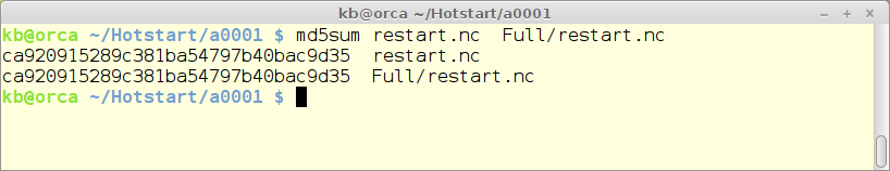
The implementation is finished. The correctness of implementation has been tested in the following way:
- A full simulation is done and the hotstart file is saved.
- A new simulation is made identical to the original one – but including a hotstart time sometime during the simulation period. The hotstart file from the final part of the simulation is saved.
- The two saved hotstart files are compared using the md5sum algorithm. If the sums are identical so are the hotstart files – and so are the simulations.
Below is shown the result from the Northern North Sea (nns_annual) standard test case. A hot-start has been injected at july 1st in the simulation year.