ParSAC
ParSAC is a sensitivity analysis and calibration tool for GOTM and fabm0d . ParSAC is written in Python.
Citable version (latest):
![]()

Introduction
ParSAC – Parallel Sensitivity Analysis and Calibration.
The calibration of complex coupled physical/bio-geochemical numerical models is a very time-consuming task typical requiring a large number of - run model -> compare with observations -> adjust paramters - cycles. The final chosen set of model parameters is the - partly - subjective judgement by the person performing the calibration and do not in anyway assure that even a small part of the global parameter space has been covered. This is mainly due to the curse of dimensionality stating that the number of realisations becomes so large that it is impossible due to resource limitations on todays computers. As an example - with only 3 model parameters and 10 subdivisions in each paramter space 1000 simulations are needed if a brute force method is applied. For models counting 10’s to 100’s a systematic search of the optimal set of parameters in the full space is impossible.
The problem sketched above is by no means unique to the field of numerical models of natural waters and a lot of research has been done during the last decades. As it is not possible to guarantee the optimal solution statistical methods have been developed. Many of these methods are based on Monte Carlo methods - i.e. a statistical method where the optimal solution is based on a choice between a number of tries. The optimal choice is based on the evaluation of an objective function calculating the performance in some way but directly comparable between model evaluations. A very important step in the Monte Carlo method is the selection of the parameter sets to be used for the model runs.
ParSAC is a tool written in Python to perform sensitivity and automatic optimization (in the Maximum Likelihood sense) of a selected set of model paramters in a GOTM simulation. The present version of ParSAC has two different methods included for finding the maximum likelyhood - Nelder-Mead (simplex) from 1965 and Differential Evolution from 1997. In addition to the actual optimisation ParSAC also provides a set of support tools for evaluating the optimization. ParSAC stores all tested parameter sets in a data-base together with the maximum-likely hood value for each of the sets. This allows for further analysis - see below for examples.
The limitations of ParSAC - and any optimization software - must be considered. ParSAC will in an objective way make an estimate on the optimal value for a set of paramters the user has specified. This is done by evaluating a function comparing model results with observations. ParSAC can not account for short-comings in the model itself - i.e. does GOTM - actually describe the processes the observations are a result of. Furthermore, ParSAC can not judge the quality of the observations provided but will use them as is. And lastly - the set of parameters to optimize for provided by the user - are they the right ones.
ParSAC is a statistical method and does not gurantee the correct solution. ParSAC comes with an estimate of the correct solution. To gain faith in the reults it is a very good idea to run a number of optimizations to see if similar results are optained between them. This behaviour is facilitated with the –repeat option shown later.
ParSAC can be run in serial and parallel mode. If the Python package parallel pythoni - pp is installed the auto-calibration task is automatically spread across available local cores. Additional configuration is possible to run on distributed memory machines as well - see the ParallelPython documentation for configuration. This makes sense only for methods supporting it.
ParSAC combines: 1) a working model (GOTM) setup with 2) a single XML formatted configuration file and 3) a set of observations to compute an optimal estimate of the included model parameters.
ParSAC operation
ParSAC is developed as a command line utility with extensive command line help support. This means that for now to get a good workflow the user must be confident working in a terminal window - independent of platform - being on Windows, Mac or Linux. Typical use will have 2 to 3 terminals open to allow for easy use of different sub-modules.
Installation
ParSAC is available from PyPI and can be installed by simply executing the command:
pip install parsac <--user>
Succes of installation can be tested by:
kb@orca ~ $ parsac -v
0.5.4
kb@orca ~ $
ParSAC usage
ParSAC is a python wrapper around a number of individual python modules. It only provides common configuration between the modules and set up infrastructure. Each of the individual modules handles their own usage and help. The very modular way ParSAC is implemented makes it easy to add new functionally to the main program.
All execution of ParSAC commands is done via the ‘parsac’ command wrapper - see the figure below.
kb@orca ~ $ parsac -h
usage: parsac [-h] [-v] {sensitivity,calibration,ensemble,service} ...

parsac - Parallel Sensitivity Analysis and Calibration

positional arguments:
  {sensitivity,calibration,ensemble,service}
    sensitivity         Sensitivity analysis
    calibration         Auto calibration
    ensemble            Ensemble simulation
    service             Service information

optional arguments:
  -h, --help            show this help message and exit
  -v, --version         show program's version number and exit
kb@orca ~ $
Each of the commands have their own help system - available like:
kb@orca ~ $ parsac sensitivity -h
usage: parsac sensitivity [-h] {sample,run,analyze} ...

positional arguments:
  {sample,run,analyze}

optional arguments:
  -h, --help            show this help message and exit
kb@orca ~ $
Main configuration file
ParSAC is configured via a xml formatted file. The example below is from the Northern North Sea annual standard set-up. The configuration file contains 5 different sections:
- transports - how are results communicated and stored
- executable path - the full path to the executable - in this case GOTM
- setup path - that path to the basic set-up
- parameters - list of parameters to use in the calibration
- observations - list of observation files - in the format shown further down
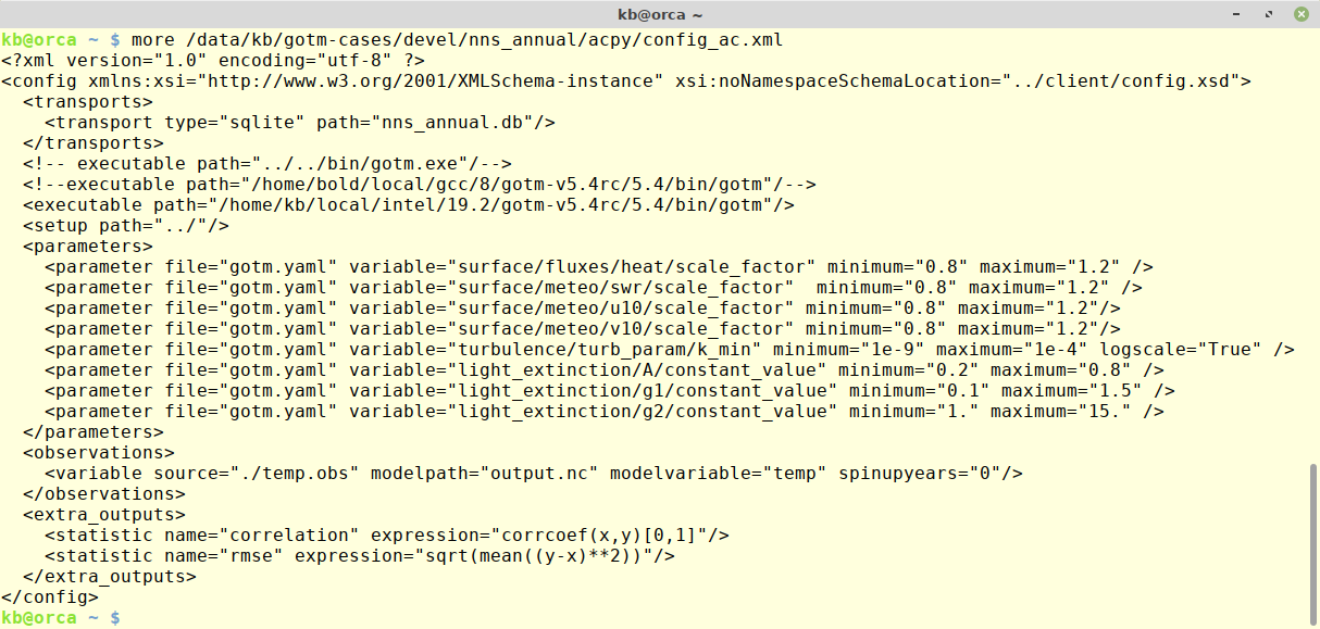
The configuration has optimized for 8 parameters in the model. The y-axis is the maximum likelihood value and the x-axes show the span for the different parameters. ParSAC supports logaritmic parameters - as the specification for k_min shows.
Parameters to optimize can specified via Fortran namelist or YAML-formatted syntax.
Database file
The autocalibration module - see the ‘run’ module - with the configuration above creates a SQLite formatted database with the results of the autocalibration tools. The specific name of this file is specified in the .xml configuration file. Most other modules with use the database file for futher processing.
Observation file format
Observations in ParSAC are read in from simple ASCII files with one variable in each file. The observation files are listed in the main configuration file and links the file to a output file and model variable. The format is very simple as seen in the figure below. Each observation consists of a time-stamp and a depth (measure from the surface).
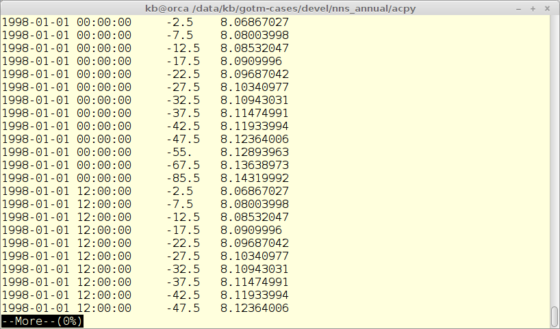
The observations are used to calculate the maximum likelihood function on which the auto-calibration is based.
Support plans
ParSAC installed from PyPi comes without any support - as shown via:
kb@orca ~ $ parsac service
Reading service from:
   /home/kb/.local/lib/python3.6/site-packages/parsac/service.txt
Section: User
  user = Unsupported version
  date = 2019-09-01
  expire = never
Section: Key
  key = dbba28d3036ddd2ea9afe5c8880194b8  -
Section: Features
  parallel = Shared
kb@orca ~ $
ParSAC support can be arranged with Bolding & Bruggeman and will depend on the type and extend of the support requested.
We provide a basic support license of ParSAC that can be obtained by contacting BB. This license will provide support to get an already configured GOTM setup ready to do sensitivity and calibration. The license does NOT provide any support in making the basic model setup. Typically the setup will be provided to BB as a .zip for us to work with. The license fee is 300,- EUR ex. VAT for a personal license.
We also offer a premium support plan that includes up to 20 days for development of tailor-made code (e.g., job submission scripts for a HPC cluster) and/or new functionality. This plan is priced at 15.000,- EUR ex. VAT. Any new functionality developed under this plan would in principle be made publicly available as part of the open source ParSAC application.
With the basic support plan the licensed wheel file is strictly personal and must under no circumstances be distributed to third parties.
With the premium support plan the licensed wheel file is institutional and must under no circumstances be distributed to third parties.
A support version of ParSAC will be provided as a wheel file and must be installed on the computer(s) using the command:
pip install <name_of_wheel_file> <--upgrade> <--user>

<--upgrade> <--user> are optional.

<--upgrade> if ParSAC is already installed on the system
<--user> if installation is not system wide
The licensed and non-licensed versions of ParSAC will produce the same results when run on the same configuration (except for differences inherent in statistical methods where you draw random numbers from probability distributions).
So what is the difference - and why should I pay for a license:
- The development work of ParSAC has been considerable and started when Jorn Bruggeman worked in Oxford as a personal tool. Since then BB have added new features and made it much more generic and user friendly.
- It is not a viable business model to develop and provide the software for free - and then in addition also provide free service.
- Further development of ParSAC will 100% depend on external funding.
- Any type of support will require a license-file with support enabled.
- The http transport method requires additional configuration. This transport method allows for doing the actual simulations on a remote cluster and obtaining results on your local computer.
The main advantage of automated sensitivity and calibration tools is time saving (and hopefully better model simulations). So if time is of any value to you - consider buying a support plan - for the time we have saved you.